Epidemics

04 Jan 2019
Author: ewd	Tags: python, diffeq, modeling, biotech

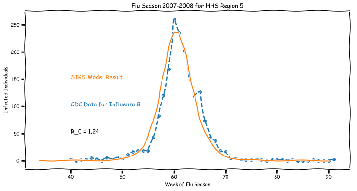
The SIR model is an example of a compartmental model used to simplify the mathematical modeling the spread of infectious diseases. While the SIR model gets a lot of attention for its use as a toy model for testing implementations, or demonstrating the power of ODEs for modeling nonlinear systems, it’s a surprisingly good fit for actual data.

SIRS Model for epidemiology of Influenza B in 2007

As a note, I’m making use of the XKCDify package for Python to generate the figures in this post. It is a deliberate design decision to give the blog a less polished feel as these are just sketches of ideas.

The data for this, and the remaining examples in this post, are drawn directly from the CDC. I’m currently focusing heavily on problems of interest to the CDC and the study of epidemics and pandemics, so this post is partially just a product of my recent data dive. The Epidemiology and Prevention Branch in the Influenza Division of the CDC has some excellent open data sets on Influenza available, so it’s pretty simple to look at different outbreaks over time.

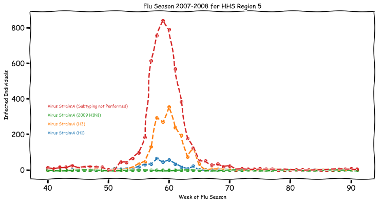
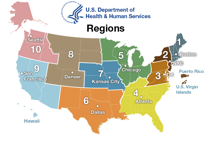
Overview of the 2007 Influenza Outbreak in Region 5

The figure above is an overview of the incidence of various strains of influenza witnessed by the CDC during 2007 for Region 5. Most of the historical data at the CDC is broken into these regions, with more recent data also available at the state level, so it requires aggregating the US as follows:

Region map as defined by HHS

The SIRS model itself is a differential equation based model aimed at modeling the dynamics of a population with the assumption that individuals begin as Susceptible, become Infected, and eventually Recover to a stage at which point they are either temporarily or permanently immune to reinfection. Modeling this system in python is a pretty straight forward task:

# N is the total population for the region, we draw it
# from the US Census data.
N = int(popData[popData['Year'] == int(popYear)][region]) #
# I0, R0, and S0 are the initial states for the SIRS
# model.  We assume a single initial case of infection.
I0 = 1
R0 = 0
S0 = N - R0 - I0

# The parameter gamma is a rate of infection.  We drew
# the estimate here from the literature.
# Rho here stands for r naught, and is the parameter
# of interest to most epidemiologists. A future post
# will discuss finding this using stochastic optimization
# techniques.
gamma = 1/3
rho = 1.24
beta = rho*gamma

def deriv(y, t, N, beta, gamma):
    S, I, R = y
    dSdt = -beta * S * I / N
    dIdt = beta * S * I / N - gamma * I
    dRdt = gamma * I
    return dSdt, dIdt, dRdt

y0 = S0, I0, R0

min = 33
max = fluData['T'].max()
t = list(range(min*7, max*7))
w = [x/7 for x in t]

ret = odeint(deriv, y0, t, args=(N, beta, gamma))
S, I, R = ret.T

# Our SIRS model predicts infected individuals, while
# the CDC data is in terms of incidence of infection
# witnessed at labs, we correct for this difference
# in measure here.
incidence_predicted = -np.diff(S[0:len(S)-1:7])
incidence_observed = fluData['B']
fraction_confirmed = incidence_observed.sum()/incidence_predicted.sum()

So how well does this model generalize? Did we just get lucky with 2007 data? Or does this very simple model apply more generally?

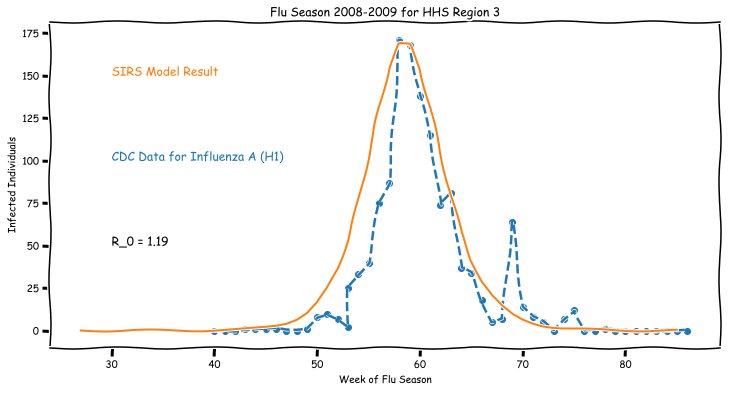
2008 Influenza A Predictions from SIRS

Sometimes very simple models have a lot of power when modeling complex systems, even when fitting real data.